How to analyze SAXS data

SAXS Processing At The Beamline

• Reduction of detector images detector images (.tif or .hdf5) to one dimensional scattering profiles (.dat) is done automatically by BioCAT’s data processing pipeline. The .dat files can be loaded directly into BioXTAS RAW for preliminary processing essentially in real time. RAW also has the funcitonality to reduce images, but this is typically not necessary.
  • RAW is a full-featured GUI-based SAXS analysis program that can do data reduction and has specialized tools for processing SEC-SAXS data. It can do analysis all the way from basic background subtraction to Guinier fits, molecular weight calculation, IFT calculation (P(r) function) using GNOM, envelope calculation using DAMMIF/N, electron density calculation using DENSS, and deconvolution of SEC-SAXS data using EFA.
  • Full written tutorials, video tutorials, a manual, and instructions for how to install RAW on your own computer can be obtained from the RAW website.
  • BioCAT users may find the section on Basic SEC-SAXS processing particularly useful.
  • Beamline scientists will provide hands-on training with RAW at the beamline
  • RAW is developed and maintained by Jesse Hopkins, a beamline scientist at BioCAT. Bugs reports, feature requests, and other RAW questions should be sent to him.
• In addition to RAW we also provide the ATSAS package (latest version), pyMOL and Chimera on the primary data analysis computer.
• There is an additional identically configured computer available for data analysis at the beamline.

Processing SEC-SAXS data

SEC-SAXS data is collected continuously as a series over the course of the elution. Data can be loaded into the Series tab in RAW, either in online mode (as eluting) or not (afterwards).

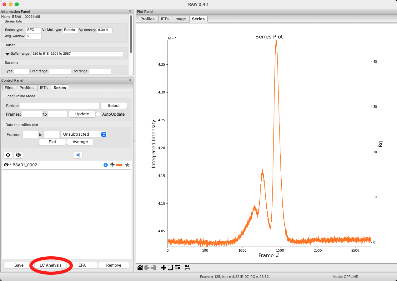
1. From the RAW series tab, select the series of interest and open the LC analysis tool:

   

2. In the LC analysis window that opens, you need to select buffer and sample regions to average. You can manually select buffer regions with the “Add Region” function. Multiple selected regions will be averaged together. Once you have selected buffer regions, hitting “Set Buffer” will average your selected frames and subtract the entire seires. Some tips for buffer selection:

   • It is generally best practice to select buffer regions where the integrated intensity is flat, and you are confident no minor species are eluting.
   • It can be helpful to check the MALS and dRI traces, if available, as they are more sensitive than SAXS.
   • Selecting both pre-elution and post-elution buffer can help correct for minor variances such as beam drift, changing effective concentrations of reductants or accumulating sheath buffer damage
   

3. Once you have selected appropriate buffer regions, select a sample region to average in a similar fashion. if possible, avoid regions where Rg, MW, etc. is changing. This may indicate the presence of multiple species, which would warrant a deconvolution method, such as EFA or REGALS. The presence of multiple species across a part of the elution can also be assessed by singular value decomopositon (SVD). Deconvolution methods available in RAW include Evolving Factor Analysis (EFA) and Regularized Alternating Least Squares (REGALS).

   

4. Once you have selected appropriate buffer and sample regions, simply hit “To Profiles Plot” and your subtracted and averaged profile will appear in the “profiles” tab. Hitting “OK” will close the LC analysis window.

   

Processing batch mode SAXS data

Batch mode data at BioCAT is collected in a continuous flow mode, and so the data presents much like an elution off a column except much shorter. These data can be loaded directly into RAW as a series, similar to SEC-SAXS data. The process of data collection is a somewhat unusual modality due to the coflow cell used at the beamline. Sample is aspirated into the needle and the needle is moved into the cell. The sheath buffer is continuously flowing through the cell. The sample is then injected from the needle. There is necessarily a short time at the start of sample injection for the stream to become fully established, i.e. at full width in the cell, and similarly a short time at the end after injection stops where the stream width tapers before fully dissipating. In between these bookends there is a constant intensity region of the data collection that represents the time where the sample is at full stream width, and this is what should be used for analysis.

1. Pre-sample buffer

2. Start of injection/signal rise

3. During injection/constant signal

4. End of injection/signal fall

5. Post-sample buffer

   

If data was collected where the coflow sheath buffer is a perfect match to the sample, processing a single series is relatively straightforward using the LC analysis tab in RAW. The process is analagous to monodisperse SEC data.

1. From the “series” tab, select the series of interest and hit the “LC analysis” button:

   

2. First, select buffer regions, book-ending the elution peak if possible, using the “Add Region” button, followed by “Set Buffer” to average the buffer frames and subtract the series:

   

3. Once you have selected a buffer region, select a sample region in the same way. It is best practice to select only from the constant concentration region, if possible. After sample region selection, “To Profiles Plot” will average the subtracted sample frames and send the subtracted and averaged profile to the profiles tab in RAW:

   

IMPORTANT: When averaging buffer and sample regions, take care to avoid large spikes in your average, as they may represent small bubbles, debris, etc.

If data was collected where the coflow sheath buffer is not a perfect (i.e. dialysis) match, then subtraction must be done using a separate injection to measure the appropriately matched buffer. Typically, the elution of the sample is clear, and initial subtraction can be performed in the same way as described in section (1). Generally, it is good practice to use the same regions for the matched buffer injection as was used for the sample – in cases where the elution is not obvious from the integrated intensity plot, this may be a necessity. In the example shown below, the sample injection on the left and the buffer on the right. In some cases, the buffer injection may be indistinguishible from the coflow sheath buffer on the integrated intensity plot.

1. For both the sample and buffer datasets, proceed with buffer and sample region selection as appropriate and then export the profiles to the main RAW window using the “To Profiles Plot” button.

   • Performing a “double subtraction,” where you subtract the contributon of the coflow buffer from both datasets, is optional. It will add noise to the final profile but in some cases can help compensate for other factors such as beam drift.
   

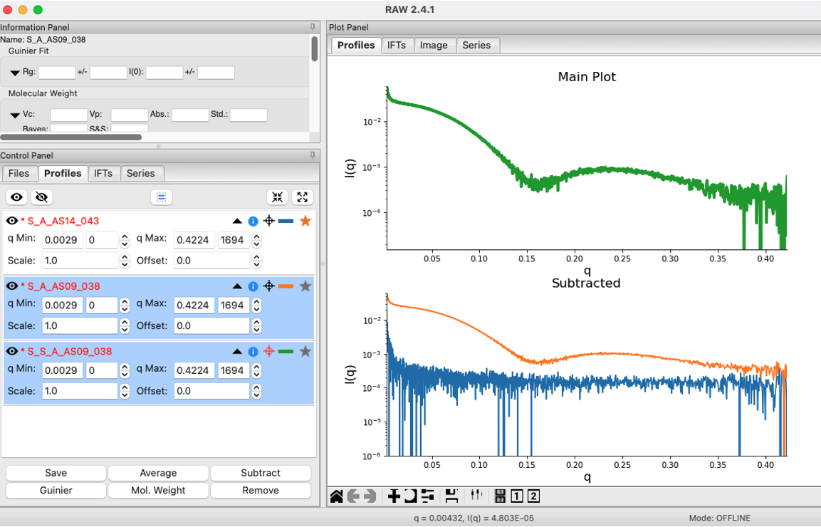
2. To obtain the fully subtracted profiles, simply star the buffer dataset (the yellow star to in the far right of the profiles tab), select the sample dataset and hit “subtract”. The fully subtracted profile will then appear in the profiles tab.

   

Further analysis

• Once you have obtained a fully subtracted profile, basic anlaysis and data validation should be performed. This can include:
  • Guinier fit
  • MW calculation to verify data quality and oligomeric state
  • P(r) calculation using GNOM and datGNOM
  • Evaluating the potential ambiguity of a 3D reconstruction using AMBIMETER to verify that a reconstruction is worth doing
  • 3D reconstruction with ab initio bead models using DAMMIF/N and average these models using DAMAVER or cluster these models using DAMCLUST
  • 3D reconstruction with ab initio electron density models using DENSS and EMAN2
• For more on what RAW can do, see the full tutorial: tutorial and tutorial videos
• Alternatively, you can use Primus or Scatter for the processing described above, except for the electron density reconstruction.

SAXS Data Processing At Home

• Users will take home all unprocessed data: .tif files and log files, as well as a RAW .cfg file. In addition, they will take home any data processed at the beamline.
• In order to carry out basic processing (images into one dimensional scattering profiles) users will need to install RAW.
  • IMPORTANT: You need version 1.5.2 or greater to process (image) data collected at BioCAT.
• Once you’ve installed RAW, make sure to load in your config file (“SAXS.cfg”) BEFORE loading any images.
  • This part of the RAW tutorial covers loading config files and how to process batch-mode samples: https://bioxtas-raw.readthedocs.io/en/latest/tutorial/s1_basic.html
  • This part of the RAW tutorial covers basic SEC-SAXS data processing: https://bioxtas-raw.readthedocs.io/en/latest/tutorial/s1_sec.html
• Please check the RAW tutorial and the RAW tutorial videos for more processing help, and reach out to use if you have any questions.
• If you’d rather use another data processing program (like Primus or ScAtter), simply load your .cfg file into RAW, select all of your images in the ‘File’ Control Panel and click ‘Quick Reduce’. This will generate .dat files from the images without loading them into RAW. These .dats are compatible with most popular SAXS software packages.

In the following two videos, Dr.s Jesse Hopkins and Kushol Gupta discuss basic and advanced SAXS data analysis (get basic slides, get advaced slides)