This provides instructions of how to collect SAXS data at the BioCAT beamline. Before comming, please ensure that you’ve read up on how to plan your experiment and that you’ve properly prepared your samples.
Before data collection
There are a few common processes:
- Every buffer you use for SEC-SAXS should be filtered and degassed. As we use a single system for SEC and SEC-MALS experiments, passing buffers through 0.1-micron filters is highly recommended. Sheath buffers can be filtered with 0.22-micron filters.
- In SEC-SAXS experiments you should reserve ~50 mL of buffer in a falcon tube. This can be used for checking concentration, diluting samples, etc. It is convenient to not have to extract this from the larger buffer bottles.
- Most samples should be spun down for 10 minutes just before measurement. Please decant into a new tube to avoid loading aggregate or debris that have spun down. Some types of samples, such as nanoparticles or micelles, should not be spun down.
Submitting actions - getting oriented
All system control, with the exception of running MALS data collection, can be done through the BioCAT Control GUI. Most relevant actions (such as column equilibration and sample submission) can be done through the automator tab. Other tabs offer finer control over individual instruments or settings, but are not necessary to interact with for standard SAXS sample submission.

To submit a sample, simply click the “add action” button. A window will pop up with a list of actions, which includes sample submission for all equilibrium modes (SEC, AF4 or batch)

Changing buffer
To change SEC buffer you must do two things. First, you need to equilibrate the column in the new buffer. Second, you need to change the coflow buffer. Both actions can be performed simultaneously through the “Equilibrate column” action in the “Add action” window as seen above. If the MALS is in-line, you must also open the purge valve on the RI instrument to allow for the cell to equilibrate. Changing buffer for batch mode only requires changing the coflow buffer, as there is no “running buffer.”
IMPORTANT: Do not change leads while flowing!
IMPORTANT: Never change directly from a buffer with salt to a storage solution of 20% ethanol, or vice versa. This could cause salt to crash out of solution and damage equipment. Always include a water equilibration step between those types of solutions.
IMPORTANT: ALways double check the column flow path and coflow inlet valve positions are correct.
Loading Samples
- For SEC-SAXS, SEC-MALS-SAXS or AF4-SAXS:
- Samples can be loaded from most standard tube or vial types using the Agilent autosampler. Typically, 1.5-mL standard Eppendof tubes are used by default.
- The middle drawer of the Agilent, denoted D2, is configured to take standard 1.5- or 2-mL Eppendorf tubes. The bottom drawer is configured for 96-well plates.
- After spinning down your sample, decant as much of the liquid as possible into a fresh tube to avoid loading any aggregate or debris that may have been spun down.
- Uncap the tube, fold back the cap and load it into the next available space in the Agilent autosampler. It is useful to sequester the cap in the space next to the tube well, so that the tube sits snugly without moving or popping up.
- Close the drawer and the incubator, search and exit the hutch.
- For batch mode SAXS:
- Load as many samples as intended into unused wells on a standard 96-well plate.
- Briefly spin down the plate using the plate centirfuge in the wet lab, to avoid injecting bubbles at the bottom of the well.
- Apply a pre-pierced plate cover, and load the plate onto the batch mode plate holder with well A1 facing the downstream/outboard corner. Insert the plastic spacer on the upstream side of the plate.
- A “change plate” utility is available in the autosampler window, or on the autosampler control itself open on the coflow control laptop (which lives on the back of the hutch table). This will move the plate motors out for easier access to the plate holder — you just need to remember to hit “OK” when finished!
Setting up data collection
Collecting SEC-SAXS or SEC-MALS-SAXS data
In the “Add Action” window, select the appropriate action for your experiment. Here, we will walk through SEC-SAXS data collection (the “Run SEC-SAXS sample” option). After selecting that option and hitting “OK”, a new window will appear, where you can change experimental parameters and the metadata that will be recorded for your measurement.
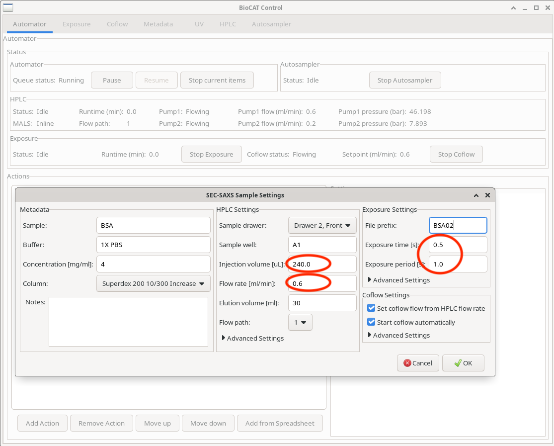
At this stage, double check your data collection parameters. The most important parameters to check are:
- That the injection volume is appropriate. It is recommended to inject 5-10 uL less than the nominal volume in the tube to avoid injecting bubbles.
- Your elution volume is sufficient. A 10/300 column has an elution volume of ~24 mL, so 25 mL is typically sufficient for capturing the entire elution, including post-buffer.
- Your exposure time and settings are appropriate for the experimental type. Typical settings for SEC- and AF4-SAXS are 0.5-second exposure time/1.0 second period.
- Your set flow rate is appropriate. Typically, we run 10/300 columns at 0.6 mL/min by default. However, some experimental conditions, such as high (>5%) glycerol buffers or low-temperature experiments may necessitate slower flow rates.
Once you hit “OK”, the sample will automatically submit unless the automator queue is paused.
IMPORTANT: If you are collecting MALS/RI data, ensure that the MALS data collection has been started before hitting “OK”, as both the MALS and SAXS data collections are triggered by an inject signal from the Agilent instrument. Please see the “Setting up MALS data collection” instructions below.
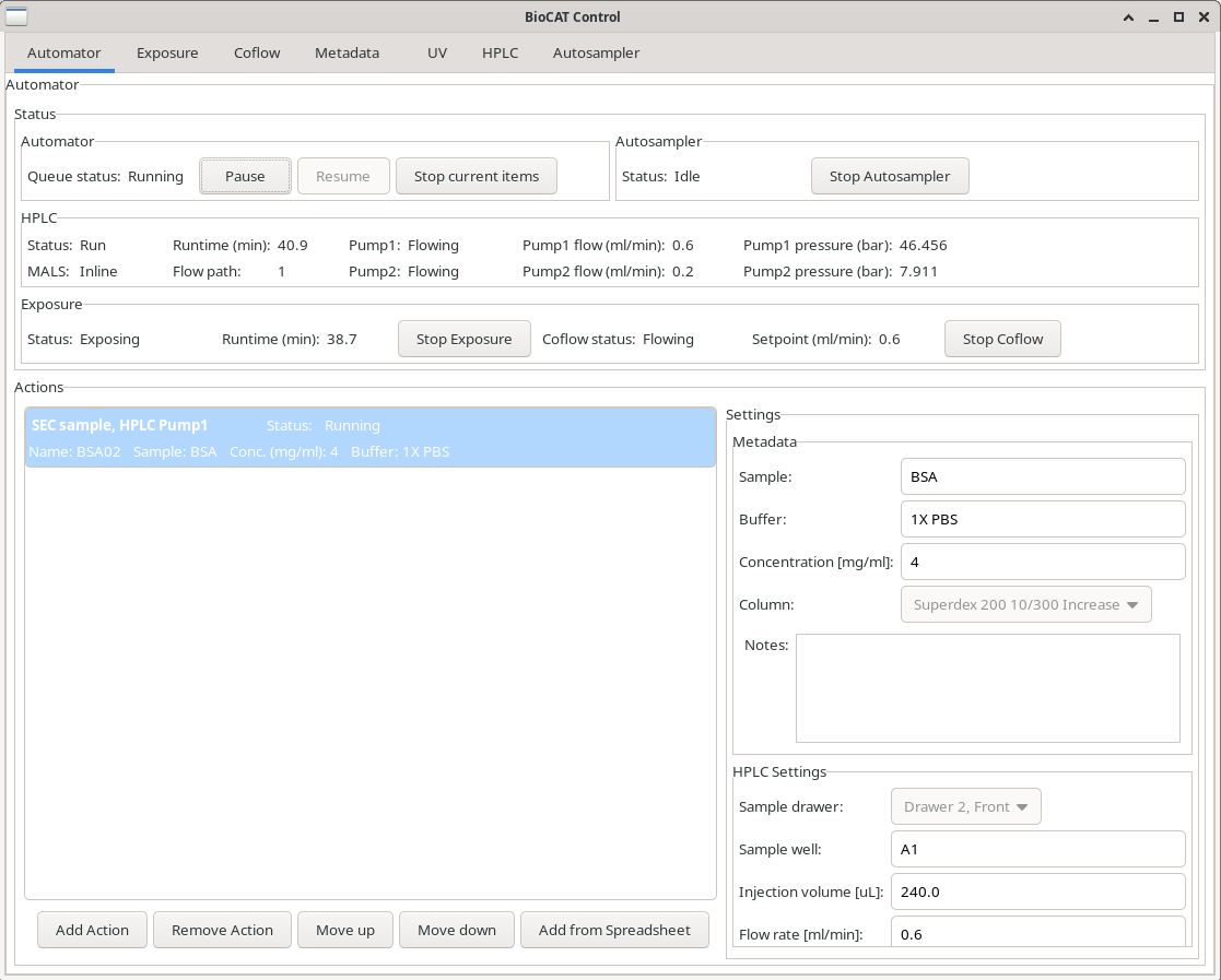
Once data collection has started, you will see a sample present in the “Actions” window, which may be running or queued. Clicking on any white space will reveal the settings that were defined when submitting the sample.
You may add additional actions in the queue, even if one is currently running. This is useful for submitting multiple samples in sequence to save time going in and out of the hutch.
Setting up MALS data collection
MALS/DLS/dRI data collection is controlled through Waters’ ASTRA software, which runs on the MALS control computer. Typically, there is a remote desktop window open to that computer (if not, please contact your beamline scientist).
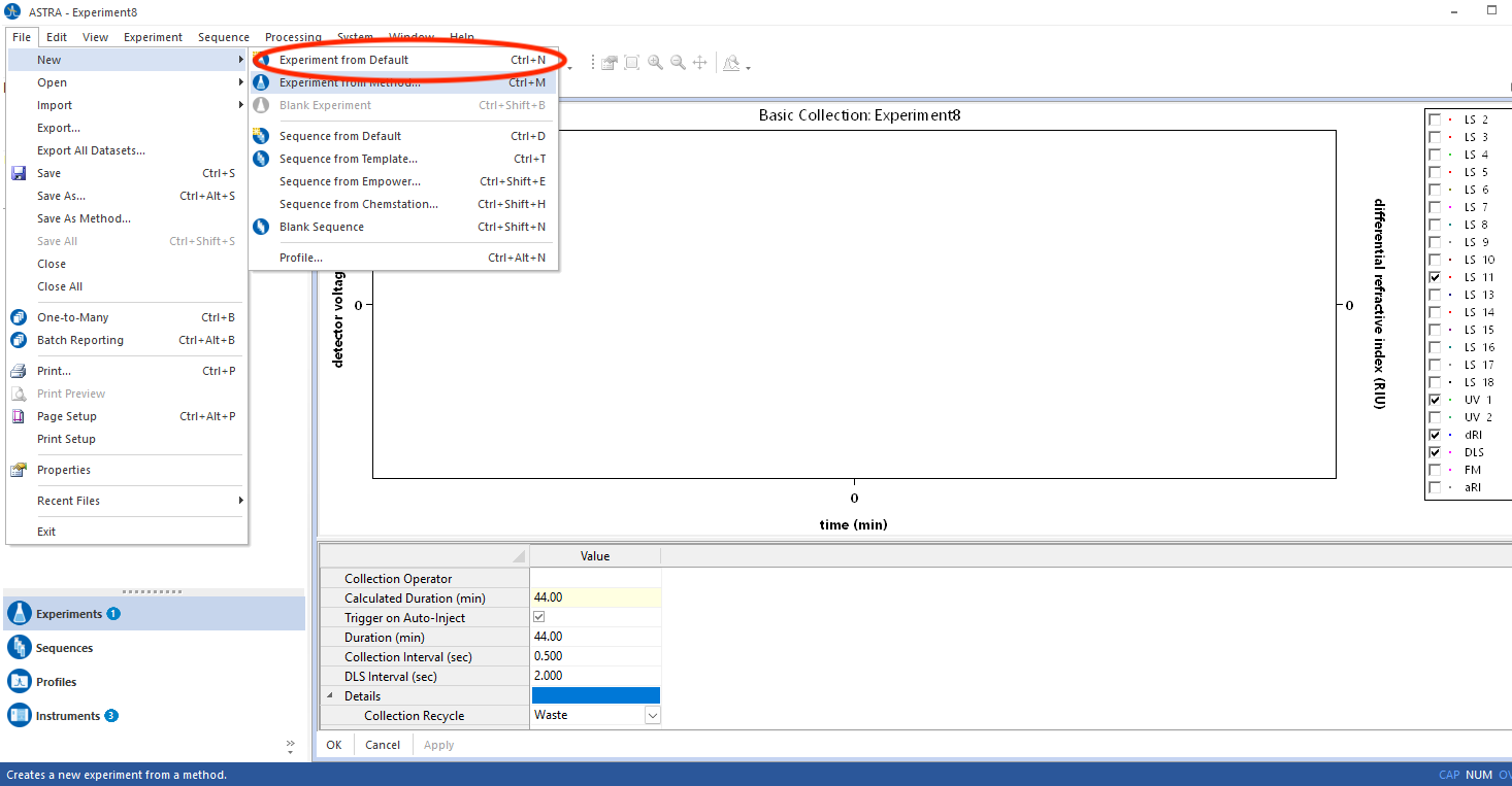
A pre-calibrated MALS data collection method is prepared as a default method at the start of every SAXS block, where band broadening and alignment are fit using a BSA standard. To start a MALS data collection, in the ASTRA software simply go to File -> New -> Experiment from Default
An experiment will then open. Expanding the experiment in the leftmost window will reveal a number of sub-tabs. It is generally a good idea to check the following:
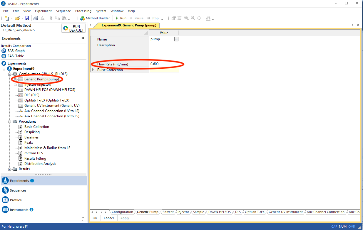
- In the “Generic pump” window, make sure your flow rate matches the set flow rate in the Biocon control (typically 0.6 mL/min for 10/300 columns)
- In the “Basic collection” window, make sure your duration is sufficient. 40 minutes is standard for a 24-mL column at 0.6 mL/min, but that may need to be extended if running at a slower flow rate.
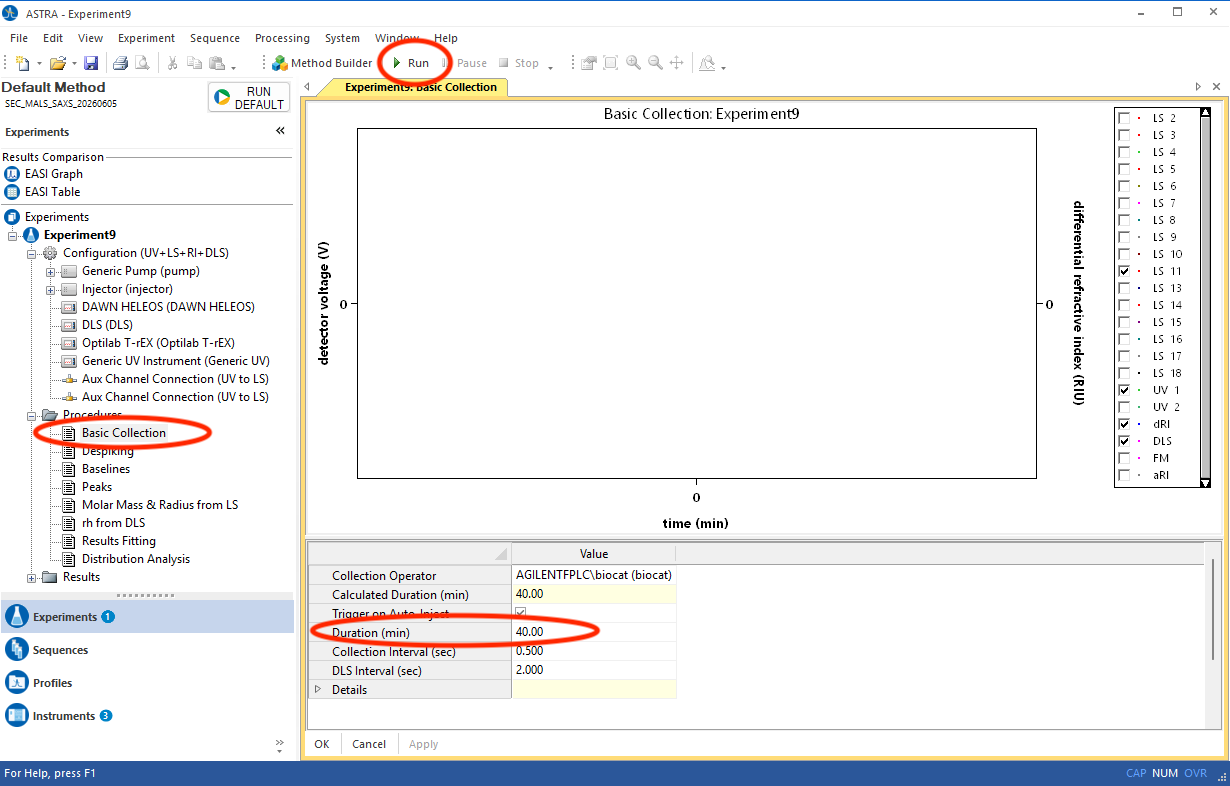
After checking parameters, it is recommended that you save your method and give it an appropriate name. Then, simply hit “run.” Text should appear in the main collection window that says “preparing for collection.” This will eventually proceed to read “waiting for auto-inject signal.” This means the MALS instruemnts are waiting for an inject mark, which is sent by the Agilent system once a sample has been injected. It is at this point that you are safe to proceed with submitting the sample for SAXS data collection.

Once MALS data collection has started, you should see some of the traces start to appear on the “Basic Collection” window. Once data collection has finished, don’t forget to save!

Setting up batch mode data collection
- In the “Add Action” window, select “submit batch mode sample.” A new window will appear, which shows the plate layout and parameters
that can be adjusted for data collection.
- Select the appropriate well and double check your exposure time and period are correct (typical settings are 0.199 second exposure time/0.2 second period).
- Check your injection volume is approrpiate. It is recommended to load 1-2 uL less than what is nominally loaded into the well, to avoid drawing up bubbles. A 30 uL well load/29 uL injection is a typical default setting.
- Hitting “OK” will automatically submit the sample. You may add additional actions in the queue, even if one is currently running.
Checking collection and inspecting data
Once data collection has started (i.e. the sample has been injected), for SEC or AF4 the status of the Agilent system will be “run.” This can be seen by opening the Ailgnet software window in the remote desktop window for the MALS control computer. It is a good idea to periodically monitor the pump pressure (this value can also be seen in the BioCat Control GUI main Automator tab or the HPLC tab, but the real-time pressure “Online Signals” plot in the Agilent control can sometimes be helpful). Generally speaking, the expected system pressure with a 10/300 column on BioCAT’s system should be between ~45 and 48 bar. If the pressure is above ~50 bar, you may need to decrease your flow rate or contact your favorite beamline scientist. The pressure alarm (stop flow) is set at 60 bar.

When data is collecting, you should be able to see the beam fluorescence off the capillary in the in-line viewer window. Occasinal page refreshes may be necessary.

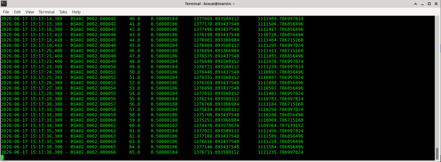
If data collection is functioning properly, there will be a terminal window where you can see the time stamp, filename, exposure time and beam intensity values scroll in real-time:
Detector image reduction is done on-the-fly, so SAXS data can be loaded directly into BioXTAS raw and processed in real-time. Both SEC and batch data are collected as series. To load online series in RAW, navitage to the “Series” tab, and hit the “Select” button in Load/Online Mode:

The “select” button will bring up a file navigator. Simply navigate to the “profiles” subdirectory of your sample folder; selecting any profile will automatically load the entire series:


Instructions for basic SAXS data analysis can be found here.
Optimizing your time
There are several things to keep in mind to help you optimize your time:
- Buffer changes can take some time. Optimize by combining samples into the same buffer as much as possible. Also make sure you know what experiments you’re doing in which buffer and do them all at once so you don’t have to re-equilibrate.
- Groups with a lot of buffer changes can pre-equilibrate columns off-line on our standalone Teledyne pumps while running other conditions.
- You should start spinning down your next sample with ~10-15 minutes left in your current run. This means starting to prepare any dilutions necessary as soon as you’ve started data collection on your current sample.
- If you’re sure all of the injection, including small molecules has eluted, you can stop your data collection early. Many users are able to stop data collection after 1 CV, and don’t need the entire 1.5 CV elution to clear the column.